When I was an undergraduate student in Nankai University, I chose a course called Data Structure and Computing Algorithms introduction from Department of Mathematics. Three years passed, I have learned a lot of other algorithms beyond the content of that class, and I found that the code I wrote at that time was kind of … duh. Never mind, this course raised my interest in machine learning at least and I really enjoyed it. In this post, I’m going to briefly review what I did in the course project: Site selection of recycle station of Nanshan District, Shenzhen, China. This project was finally presented in class on 2012-12-17 and the project was originally in a mathematical modeling contest.
In Nanshan District, there are 38 waste collection stations. Waste from every residential and commercial unit will be sent to the 38 waste collection everyday. Waste can be divided as two parts: recyclable and un recyclable. People in every waste collection station will separate the waste and send the recyclable waste to recycle station and send the unrecyclable waste to waste-to-energy burning plant located at the southwest part of Nanshan District. Thus, the project mainly consists of two problems:
- Since we have 2 sizes of recycle stations, big and small, how many and what kind of recycle stations are needed? Where should we set the waste recycle station to minimize the cost of transportation?
- If we’re going to use one big truck from one collection station to transport unrecyclable waste from its original plant and other unrecylcable waste from some other collection station along its road to burning plant, what will be his optimal road?
Problem 1 Location of Recycle Station
The map of Nanshan District is: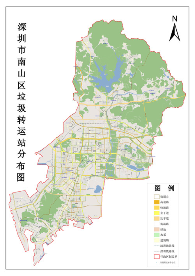
And the list of collection station looks like this:
| Sequence | Name | Position | Operation Corporation | Quantity |
|---|---|---|---|---|
| 1 | 9th Street Station | Shen Nan Ave beside Nantou Middle School | De Ying Li Corporation | 20 |
| 2 | Yu Quan Station | Yu Quan Rd and Bao Long Rd Crossing | De Ying Li Corporation | 25 |
| …. | ….. | ……….. | ………………….. | ……… |
| 38 | Tang Lang Station | In Tang Lang Industrial Zone | Recycling Main Corporation | 10 |
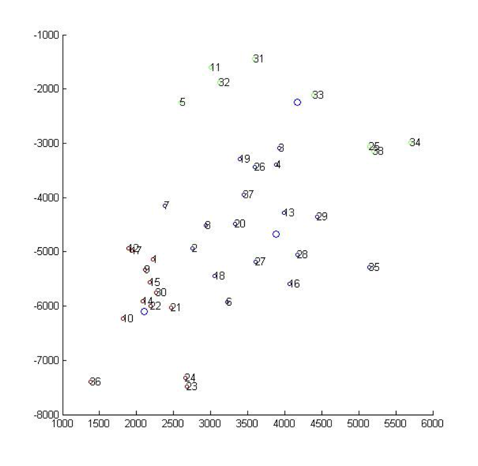
We first marked every waste collection station manually according to the position described in the above list on the map. And put the map into mathematica to get the coordinates of every collection station like this:
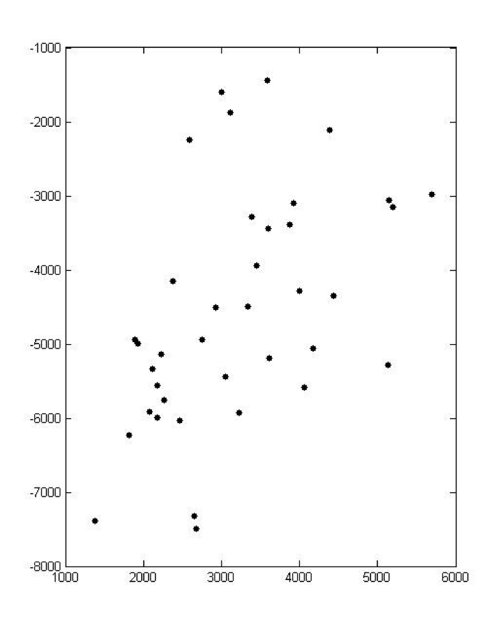
And the list of coordinates of collection is as following, where
| Sequence | X | Y | C |
|---|---|---|---|
| 1 | 2225 | -5138 | 20 |
| 2 | 2749 | -4940 | 25 |
| … | … | …. | |
| 38 | 5195 | -3147 | 10 |
Problemt 1.1 Estimation of Cost
To solve the problem of how many big or small recycle station to build, we did a simple estimation. The condition we have at that time is:
| Variable | Number |
|---|---|
| The Area of Nanshan District | 182 km^2 |
| Recyclable Waste in collection station | 536 ton/day |
| Truck Load | 10 ton |
| Truck fuel consumption per ton | 27.5 L/100km |
| Fuel Price | 7.5 RMB/L |
| Big Station Treatment Capacity | 200 ton/day |
| Small Station Treatment Capacity | 0.25 ton/day |
| Big Station Building Cost | 45 Million RMB |
| Small Station Building Cost | 0.28 Million RMB |
| Big Station Treatment Cost | 150 RMB/ton |
| Small Station Treatment Cost | 200 RMB/ton |
Thus, according the data of each waste collection station and the data above, we will have an estimation below:
| Station | Cost |
|---|---|
| No. of Small Station : 2144 | 6.4 * 10^8 RMB/year |
| No. of Big Station: 1 and No. of Small Station: 1344 | 4.56 * 10^8 RMB/year |
| No. of Big Station: 2 and No. of Small Station: 544 | 2.58 * 10^8 RMB/year |
| No. of Big Station: 3 | 1.64 * 10^8 RMB/year |
Even if we think the Nanshan District is a round area and we put every collection station at the border with the recycle station at the center, we still find that the difference between every two condition above in the table is almost 30 times of the transportation cost every year. Thus, we don’t need to consider transportation cost when deciding what kinds of stations to build and the decision is to build 3 big stations since this results in the least cost every year.
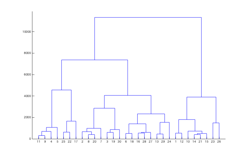
Problem 1.2 Clustering
Since we found 3 big stations is the answer, we then use hierarchical cluster analysis to cluster the collection stations into 3 group and then by finding the barycenter of each group we can determine which location to build the recycle station. As for the clustering analysis, we use a agglomerative way to divide. We first regards the 38 collection stations as in their own clusters, and limits the distance between each clusters and the way to calculate distance between each collection station. Then we combine every 2 “adjacent” stations to one cluster, and calculate the distance between this new cluster to other clusters, and so on, until we can see on the graph that the collection stations are divided into 3 groups.
Matlab code is as following:
1 | clc; data=xlsread('Book.xls',1); x=data(:,3); y=data(:,4); c=data(:,5); XY=[x y]; Z = linkage(XY,'ward','euclidean','savememory','on'); c = cluster(Z,'maxclust',3); scatter(x,y,10,c); dendrogram(X); hold on; |
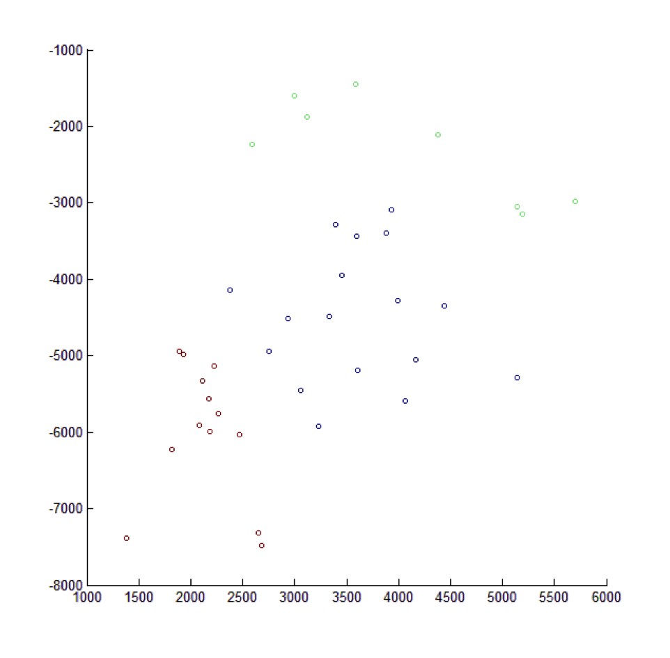
Then the map after clustering is as following, with different groups are in different color:
And the relationship of clustering is as follows:
To find the barycenter within each group by regarding the treatment capacity as their “weight”, we can find the center depicted in the map:
And the function to find the barycenter is:
1 | function cg=barycenter(mass,coord) % mass is the treatment capacity % coord is the coordinates of every station dm=size(coord); m=dm(1); n=dm(2); cg=zeros(1,n); tmass=sum(mass); for j=1:m for i=1:n cg(i)=cg(i)+mass(j)*coord(j,i); end end cg=cg/tmass; |
Problem 2 Route to Burning Plant
To make this route we use Dijkstra to find the shortest route for a truck if it starts from one station to the final station. For economic concern, we assume the truck should better go to other stations before it finally reaches the burning plant since everyday the unrecyclable waste in one station usually will not meet the upper limit of a truck’s capacity and thus the truck should go to multiple stations to save fuel for other trucks.
Next is an example code of one truck from No.31 station to Burning Plant. Since we regard the Burning Plant as the No.39 station, we put 39 as the end in the following program.
1 | clc; clear; close all; points = load(‘Points.txt'); lines = load('Lines.txt'); A = ones(size(points, 1))*Inf; for i = 1 : size(A, 1) A(i, i) = 0; end figure(‘NumberTitle’, ‘off’, ‘Name’, ‘ Connections', ... 'Color', 'w', 'units', 'normalized'); hold on; axis on; plot(points(:, 2), points(:, 3), 'g.','MarkerSize',20); for i=1:length(points(:,2)) str=[num2str(i)]; text(points(i,2),points(i,3),str,'FontSize',10) end for i = 1 : size(lines, 1) temp = lines(i, :); pt1 = points(temp(2), 2 : end); pt2 = points(temp(3), 2 : end); len = norm([pt1(1)-pt2(1), pt1(2)-pt2(2)]); A(temp(1), temp(2)) = len; plot([pt1(1) pt2(1)], [pt1(2) pt2(2)], 'k-', 'LineWidth', 1); end s = 31; % Begin e = 39; % End [dist,path] = dijkstra2(points,lines,s,e); fprintf('\n Use Dijkstra the Min Distance is: %.5f \n', dist); fprintf('\n Use Dijkstra the Min Distance path is: \n'); disp(path); |
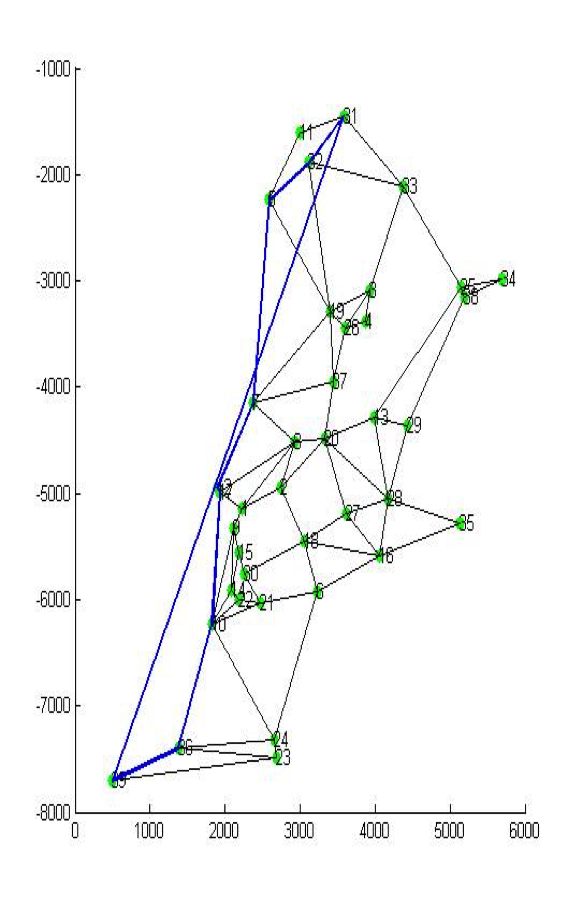
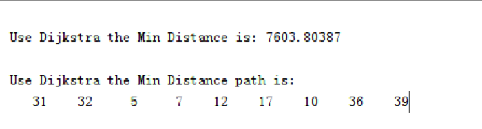
As the output indicates, if we are going to the Burning Plant from No.31 station, we should pass No. 32, No.5, No.7, No.12, No.17, No.10, No.36.
The dijkstra algorithm function is:
1 | function [dist,path] = dijkstra(nodes,segments,start_id,finish_id) % initializations node_ids = nodes(:,1); [num_map_pts,cols] = size(nodes); table = sparse(num_map_pts,2); shortest_distance = Inf(num_map_pts,1); settled = zeros(num_map_pts,1); path = num2cell(NaN(num_map_pts,1)); col = 2; pidx = find(start_id == node_ids); shortest_distance(pidx) = 0; table(pidx,col) = 0; settled(pidx) = 1; path(pidx) = {start_id}; if (nargin < 4) % compute shortest path for all nodes while_cmd = 'sum(~settled) > 0'; else % terminate algorithm early while_cmd = 'settled(zz) == 0'; zz = find(finish_id == node_ids); end while eval(while_cmd) % update the table table(:,col-1) = table(:,col); table(pidx,col) = 0; % find neighboring nodes in the segments list neighbor_ids = [segments(node_ids(pidx) == segments(:,2),3); segments(node_ids(pidx) == segments(:,3),2)]; % calculate the distances to the neighboring nodes and keep track of the paths for k = 1:length(neighbor_ids) cidx = find(neighbor_ids(k) == node_ids); if ~settled(cidx) d = sqrt(sum((nodes(pidx,2:cols) - nodes(cidx,2:cols)).^2)); if (table(cidx,col-1) == 0) || ... (table(cidx,col-1) > (table(pidx,col-1) + d)) table(cidx,col) = table(pidx,col-1) + d; tmp_path = path(pidx); path(cidx) = {[tmp_path{1} neighbor_ids(k)]}; else table(cidx,col) = table(cidx,col-1); end end end % find the minimum non-zero value in the table and save it nidx = find(table(:,col)); ndx = find(table(nidx,col) == min(table(nidx,col))); if isempty(ndx) break else pidx = nidx(ndx(1)); shortest_distance(pidx) = table(pidx,col); settled(pidx) = 1; end end if (nargin < 4) % return the distance and path arrays for all of the nodes dist = shortest_distance'; path = path'; else % return the distance and path for the ending node dist = shortest_distance(zz); path = path(zz); path = path{1}; end end |
Discussion
Looking back to this project, I did find some modifications that can be made, such as changing the euclidean distance to manhattan distance or trying to figure out a dynamic way to solve how many trucks are needed everyday to transport unrecyclable waste to Burning Plant.