Machine Learning Study Notes - Regularized Logistic Regression

When I was taking Applied Econometrics Course at Duke University, I learned logistic regression as a regression method, the dependent variable of which is cases such as people smoke or not. In econometrics modeling, what economists consider most is whether the model makes economic sense or not with maybe omitted variables or endogeneity. However, when dealing with large data sets with handreds or thousands of variables, we need to consider the issue of overfitting, which occurs when the machine learning model describes random error instead of actual relationship.

To solve overfitting, one common method is to regularize model. Regularization). Continuing with gradient descent, to regularize, we can add another term at the tail of original cost function and gradient descent function. Add this term, $$${\lambda \over 2m} \theta^2$$$, to cost function and $$${\lambda \over m } \theta$$$ to gradient function. This is the form of L2 regularization. According to wikipedia, L1 regularization is often preferred because it produces sparse models and thus performs feature selection within the learning algorithm, but since the L1 form is not differentiable, and can’t have a closed form, I use L2 form here.

My regularized cost function originally looks like this, which is also a good example of including for-loop in Matlab(which is bad):

function [J, grad] = costFunctionReg(theta, X, y, lambda)

   m = length(y); % number of training examples
   J = 0;
   grad = zeros(size(theta));
   g = sigmoid(X*theta);
   n = length(theta);

   J = J = (1/m)*sum(-y'*log(g)-(1-y)'*log(1-g)) + lambda/(2*m)*theta(2:n,1)'*theta(2:n,1) ;
   grad(1) = (1/m)*sum(transpose(X(:,1))*(g-y))

   for i = 2:n
   grad(i) = (1/m)*sum(transpose(X(:,i))*(g-y))+ lambda/m *theta(i);
    end

end

Since matlab calculates based on matrix, we should avoid for-loop as much as possible. One useful tool to vectorize for loop is to use element-wise multiplication operation (.*) and sum. Modify the above function with vectorization:

function [J, grad] = lrCostFunction(theta, X, y, lambda)

   m = length(y); % number of training examples
   J = 0;
   grad = zeros(size(theta));

   J = 1/m * sum(-y.*log(sigmoid(X*theta))-(ones(size(y),1)-y).*log(1-sigmoid(X*theta))) + lambda/(2*m)*theta(2:size(theta))'*theta(2:size(theta));                                                                               
   grad(1)= 1/m * (sigmoid(X*theta)-y)'*X(:,1);
                       
   grad(2:size(theta)) = 1/m * ((sigmoid(X*theta)-y)'*X(:,2:size(theta)))'+ lambda/m*theta(2:size(theta)) ;

   grad = grad(:);

end

After completing cost function, we can write in the main.m file to use fminuncto calculate $$$\theta$$$ and then predict accuracy on training set:

initial_theta = zeros(size(X, 2), 1);
lambda = 0.1;

% Set Options
options = optimset('GradObj', 'on', 'MaxIter', 400);

% Optimize
[theta, J, exit_flag] = ...
	fminunc(@(t)(costFunctionReg(t, X, y, lambda)), initial_theta, options);

p = predict(theta,X);
mean(double(p==y))*100

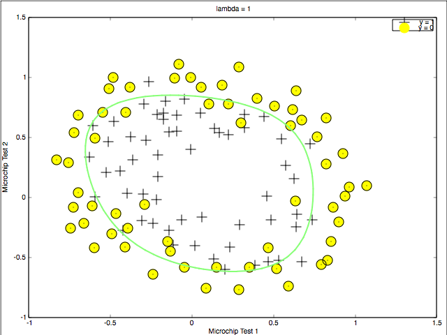
The accuracy for this project is 83%. As for logistic regression, the function of predict is like:

function p = predict(theta, X)

m = size(X, 1); % Number of training examples
p = zeros(m, 1);
for i = 1:m
    if (sigmoid(X(i,:)*theta) >= 0.5)
         p(i)= 1;
    else
         p(i)= 0;
end
                                       
end