Since I was studying Machine Learning on coursera.org, I had an idea of putting my thoughts during the study on my personal website: sunnylinmy.github.io (or mengyanglin.com). And the first course of Machine Learning is Gradient Descent.
In econometrics, the most common way to build model for forecasting is to use linear model first. After writing down the basic formula of linear model
$$$y=\theta_0+\theta_1 x_1+…+\theta_n x_n$$$ ,
one may consider the OLS be the best way to estimate $$$\theta_0$$$ and $$$\theta_1$$$ . As we all know, ordinary least squares method is achieved by minimizing the differences between the observed responses and the responses predicted by the linear approximation of the data, which is
$$${h_\theta(x^{(i)})=\hat{\theta_0} + \hat{\theta_1} x_1 +…+\hat{\theta_n} x_n}$$$ .
And the differences are $$$J(\theta0,\theta_1,…,\theta_n}) = 1/(2m) \sum({h\theta (x^{(i)})} - y^{(i)})^2$$$ .
Surely you can use functions embedded in R or Matlab to estimate the parameters very fast. However, how does embedded function in R or Matlab or other software minimize the cost function (indicated as the differences above) to calculate the parameters? One way is to use gradient descent.
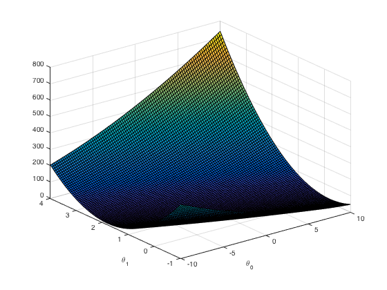
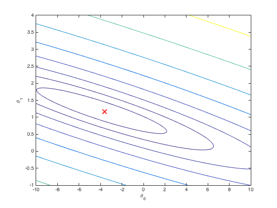
The main idea of gradient descent is that one starts with a guess of $$${\theta_0, \theta_1,…\theta_n}$$$ and change every $$$\theta$$$ a little bit by some rule every time and calculate corresponding cost function every time. Hopefully, the cost function result will become smaller and smaller (i.e. converge) and thus we will get a local minimum. And the $$${\theta_0, \theta_1,…\theta_n}$$$ at that time are the $$$\theta$$$ s we want.
The some rule we need to change theta every time is:
$$$\theta_j = \theta_j - \alpha { \partial \over \partial \theta_j} J(\theta_0, \theta_1, …\theta_n)$$$.
(The reason we use this rule is $$$J(\theta_0,\theta_1,…,\theta_n)$$$ decreases fastest if one goes from original $$$\theta$$$ s in the direction of the negative gradient of J at $$$\theta$$$ s. And this is also why this rule called gradient descent.)
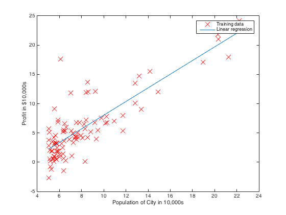
For example, we use matlab to do gradient descent. This example is from the first programming assignment of Machine Learning Course by Professor Andrew Ng on coursera.org. In the following code, we use theta to represent $$$\theta$$$ , computeCost to represent $$$J(\theta_0,\theta_1,…\theta_n)$$$.
Load Data
1 | data = load('yourdata.txt'); X = data(:,1); y = data(:,2); m = length(y); |
Use Gradient Descent to Calculate parameters
1 | X = [ones(m, 1), data(:,1)]; % Add a column of ones to x theta = zeros(2, 1); % initialize fitting parameters % Some gradient descent settings iterations = 1500; alpha = 0.01; % compute and display initial cost computeCost(X, y, theta) % run gradient descent theta = gradientDescent(X, y, theta, alpha, iterations); |
Thus, we need to write two functions: computeCost and gradientDescent function.
computeCost
1 | function J = computeCost(X, y, theta) J= 0.5*1/m*sum((X*theta-y).^2) end |
gradientDescent
1 | function [theta, J_history] = gradientDescent(X, y, theta, alpha, num_iters) m = length(y); % number of training examples J_history = zeros(num_iters, 1); for iter = 1:num_iters cost = X'*((X*theta)-y); theta = theta - ((alpha/m)*cost); J_history(iter) = computeCost(X, y, theta); end end |
The matlab code will print out 1500 lines of cost function results and when you see the J turn to be steady, the corresponding thetas are the thetas wanted. Furthermore, if we set a tolerance rate and if-else conditions, we don’t need to print out that many Js.
Following is the graph of cost J s and corresponding $$$\theta$$$ s.